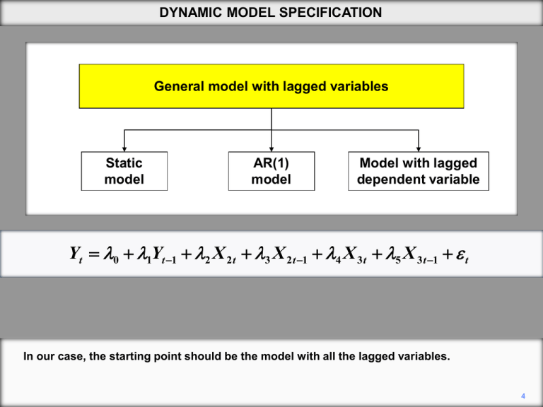
DYNAMIC MODEL SPECIFICATION
General model with lagged variables
Static
model
AR(1)
model
Model with lagged
dependent variable
Yt  0  1Yt 1  2 X 2 t  3 X 2 t 1  4 X 3 t  5 X 3 t 1   t
In our case, the starting point should be the model with all the lagged variables.
4
DYNAMIC MODEL SPECIFICATION
General model with lagged variables
Static
model
AR(1)
model
Model with lagged
dependent variable
Yt  0  1Yt 1  2 X 2 t  3 X 2 t 1  4 X 3 t  5 X 3 t 1   t
1  3  5  0
Having fitted it, we might be able to simplify it to the static model, if the lagged variables
individually and as a group do not have significant explanatory power.
5
DYNAMIC MODEL SPECIFICATION
General model with lagged variables
Static
model
AR(1)
model
Model with lagged
dependent variable
Yt  0  1Yt 1  2 X 2 t  3 X 2 t 1  4 X 3 t  5 X 3 t 1   t
3  12
5  14
If the lagged variables do have significant explanatory power, we could perform a common
factor test and see if we could simplify the model to an AR(1) specification.
6
DYNAMIC MODEL SPECIFICATION
General model with lagged variables
Static
model
AR(1)
model
Model with lagged
dependent variable
Yt  0  1Yt 1  2 X 2 t  3 X 2 t 1  4 X 3 t  5 X 3 t 1   t
 3  5  0
Sometimes we may find that a model with a lagged dependent variable is an adequate
dynamic specification, if the other lagged variables lack significant explanatory power.
7
DYNAMIC MODEL SPECIFICATION
Model with lagged variables
AR(p)
DL(q)
ADL(p,q)
In our case, the starting point should be the model with all the lagged variables.
4
DYNAMIC MODEL SPECIFICATION
General model with lagged variables
AR(p)
DL(q)
ADL(p,q)
Yt  0  1Yt 1  ...   pYt  p   t
The model includes lags of the explained variable.
5
DYNAMIC MODEL SPECIFICATION
General model with lagged variables
AR(p)
DL(q)
ADL(p,q)
Yt  0   0 X t  1 X t 1   2 X t  2  ...   q X t  q   t
The model includes lags of the independent variable.
6
DYNAMIC MODEL SPECIFICATION
General model with lagged variables
AR(p)
DL(q)
ADL(p,q)
Yt  0  1Yt 1  ...   pYt  p   0 X t  1 X t 1  ...   q X t  q   t
The model includes lags of the dependent and independent variables.
7
AUTOCORRELATION
Y
1
X
In the graph above, positive values tend to be followed by positive ones, and negative
values by negative ones. Successive values tend to have the same sign. This is described
as positive autocorrelation.
2
AUTOCORRELATION
Y
1
X
In this graph, positive values tend to be followed by negative ones, and negative values by
positive ones. This is an example of negative autocorrelation.
3
AUTOCORRELATION
Yt   1   2 X t  ut
First-order autoregressive autocorrelation: AR(1)
ut  ut 1   t
A particularly common type of autocorrelation, at least as an approximation, is first-order
autoregressive autocorrelation, usually denoted AR(1) autocorrelation.
8
AUTOCORRELATION
Yt   1   2 X t  ut
First-order autoregressive autocorrelation: AR(1)
ut  ut 1   t
Fifth-order autoregressive autocorrelation: AR(5)
ut  1ut 1   2 ut 2   3 ut 3   4 ut 4   5 ut 5   t
Here is a more complex example of autoregressive autocorrelation. It is described as fifthorder, and so denoted AR(5), because it depends on lagged values of ut up to the fifth lag.
8
AUTOCORRELATION
Yt   1   2 X t  ut
First-order autoregressive autocorrelation: AR(1)
ut  ut 1   t
Fifth-order autoregressive autocorrelation: AR(5)
ut  1ut 1   2 ut 2   3 ut 3   4 ut 4   5 ut 5   t
Third-order moving average autocorrelation: MA(3)
ut  0 t  1 t 1  2 t 2  3 t 3
The other main type of autocorrelation is moving average autocorrelation, where the
disturbance term is a linear combination of the current innovation and a finite number of
previous ones.
8
AUTOCORRELATION
Yt   1   2 X t  ut
First-order autoregressive autocorrelation: AR(1)
ut  ut 1   t
Fifth-order autoregressive autocorrelation: AR(5)
ut  1ut 1   2 ut 2   3 ut 3   4 ut 4   5 ut 5   t
Third-order moving average autocorrelation: MA(3)
ut  0 t  1 t 1  2 t 2  3 t 3
This example is described as third-order moving average autocorrelation, denoted MA(3),
because it depends on the three previous innovations as well as the current one.
8
AUTOCORRELATION
ut  ut 1   t
3
2
1
0
1
-1
-2
-3
We will now look at examples of the patterns that are generated when the disturbance term
is subject to AR(1) autocorrelation. The object is to provide some bench-mark images to
help you assess plots of residuals in time series regressions.
9
AUTOCORRELATION
ut  ut 1   t
3
2
1
0
1
-1
-2
-3
We will use 50 independent values of , taken from a normal distribution with 0 mean, and
generate series for u using different values of .
10
AUTOCORRELATION
ut  0.0ut 1   t
3
2
1
0
1
-1
-2
-3
We have started with  equal to 0, so there is no autocorrelation. We will increase 
progressively in steps of 0.1.
11
AUTOCORRELATION
ut  0.1ut 1   t
3
2
1
0
1
-1
-2
-3
( = 0.1)
12
AUTOCORRELATION
ut  0.2ut 1   t
3
2
1
0
1
-1
-2
-3
( = 0.2)
13
AUTOCORRELATION
ut  0.3ut 1   t
3
2
1
0
1
-1
-2
-3
With  equal to 0.3, a pattern of positive autocorrelation is beginning to be apparent.
14
AUTOCORRELATION
ut  0.4ut 1   t
3
2
1
0
1
-1
-2
-3
( = 0.4)
15
AUTOCORRELATION
ut  0.5ut 1   t
3
2
1
0
1
-1
-2
-3
( = 0.5)
16
AUTOCORRELATION
ut  0.6ut 1   t
3
2
1
0
1
-1
-2
-3
With  equal to 0.6, it is obvious that u is subject to positive autocorrelation. Positive
values tend to be followed by positive ones and negative values by negative ones.
17
AUTOCORRELATION
ut  0.7ut 1   t
3
2
1
0
1
-1
-2
-3
( = 0.7)
18
AUTOCORRELATION
ut  0.8ut 1   t
3
2
1
0
1
-1
-2
-3
( = 0.8)
19
AUTOCORRELATION
ut  0.9ut 1   t
3
2
1
0
1
-1
-2
-3
With  equal to 0.9, the sequences of values with the same sign have become long and the
tendency to return to 0 has become weak.
20
AUTOCORRELATION
ut  0.95ut 1   t
3
2
1
0
1
-1
-2
-3
The process is now approaching what is known as a random walk, where  is equal to 1 and
the process becomes nonstationary. The terms ‘random walk’ and ‘nonstationary’ will be
defined in the next chapter. For the time being we will assume |  | < 1.
21
AUTOCORRELATION
ut  0.0ut 1   t
3
2
1
0
1
-1
-2
-3
Next we will look at negative autocorrelation, starting with the same set of 50 independently
distributed values of t.
22
AUTOCORRELATION
ut  0.3ut 1   t
3
2
1
0
1
-1
-2
-3
We will take larger steps this time.
23
AUTOCORRELATION
ut  0.6ut 1   t
3
2
1
0
1
-1
-2
-3
With  equal to –0.6, you can see that positive values tend to be followed by negative ones,
and vice versa, more frequently than you would expect as a matter of chance.
24
AUTOCORRELATION
ut  0.9ut 1   t
3
2
1
0
1
-1
-2
-3
Now the pattern of negative autocorrelation is very obvious.
25
TESTS FOR AUTOCORRELATION I: BREUSCH–GODFREY TEST
Breusch–Godfrey test
k
Yt   1    j X jt  ut
j 2
k
q
j2
s 1
et   1    j X jt    s et  s
Test statistic: nR2, distributed as c2(q)
Under the null hypothesis of no autocorrelation, nR2 has a chi-squared distribution with q degrees
of freedom.
20
Copyright Christopher Dougherty 2013
These slideshows may be downloaded by anyone, anywhere for personal use.
Subject to respect for copyright and, where appropriate, attribution, they may be
used as a resource for teaching an econometrics course. There is no need to
refer to the author.
The content of this slideshow comes from Section 12.1 of C. Dougherty,
Introduction to Econometrics, fourth edition 2011, Oxford University Press.
Additional (free) resources for both students and instructors may be
downloaded from the OUP Online Resource Centre
http://www.oup.com/uk/orc/bin/9780199567089/.
Individuals studying econometrics on their own who feel that they might benefit
from participation in a formal course should consider the London School of
Economics summer school course
EC212 Introduction to Econometrics
http://www2.lse.ac.uk/study/summerSchools/summerSchool/Home.aspx
or the University of London International Programmes distance learning course
20 Elements of Econometrics
www.londoninternational.ac.uk/lse.
2013.03.04