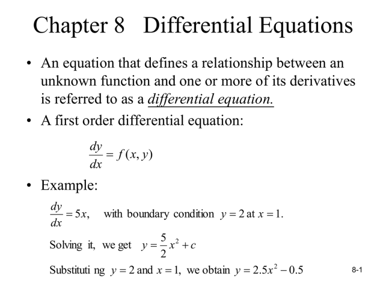
Chapter 8 Differential Equations
• An equation that defines a relationship between an
unknown function and one or more of its derivatives
is referred to as a differential equation.
• A first order differential equation:
dy
 f ( x, y )
dx
• Example:
dy
 5 x,
dx
with boundary condition y  2 at x  1.
5 2
Solving it, we get y  x  c
2
Substituti ng y  2 and x  1, we obtain y  2.5 x 2  0.5
8-1
• Example:
dy
 c( y  x)
dx
• A second-order differential equation:
d2y
dy
 f ( x, y , )
2
dx
dx
• Example:
y ' '  2 x  xy  y '
8-2
Taylor Series Expansion
• Fundamental case, the first-order ordinary differential
equation:
dy
 f ( x)
dx
subject to y  y0 at x  x0
Integrate both sides

y
y0
x
dy   f ( x )dx
x0
x
or y  g ( x )  y0   f ( x )dx
x0
• The solution based on Taylor series expansion:
( x  x0 )2
y  g ( x )  g ( x0 )  ( x  x0 ) g ' ( x ) 
g ' ' ( x0 )  ...
2!
where y0  g ( x0 ) and g ' ( x0 )  f ( x0 )
8-3
Example : First-order Differential
Equation
Given the following differential equation:
dy
 3 x 2 such that y  1 at x  1
dx
The higher-order derivatives:
d2y
 6x
2
dx
d3y
6
3
dx
dny
 0 for n  4
n
dx
8-4
The final solution:
dy ( x  1)2 d 2 y ( x  1)3 d 3 y
g ( x )  1  ( x  1) 

2
dx
2! dx
3! dx 3
( x  1) 2
( x  1)3
2
 1  ( x  1)( 3x0 ) 
(6 x0 ) 
(6)
2!
3!
 1  3( x  1)  3( x  1)2  ( x  1)3
where x0  1
8-5
Table: Taylor Series Solution
x
One Term
Two Terms Three Terms Four Terms
1
1
1
1
1
1.1
1
1.3
1.33
1.331
1.2
1
1.6
0.72
1.728
1.3
1
1.9
2.17
2.197
1.4
1
2.2
2.68
2.744
1.5
1
2.5
3.25
3.375
1.6
1
2.8
3.88
4.096
1.7
1
3.1
4.57
4.913
1.8
1
3.4
5.32
5.832
1.9
1
3.7
6.13
6.859
2
1
4
7
8
8-6
8-7
General Case
• The general form of the first-order ordinary
differential equation:
dy
 f ( x, y )
dx
subject to y  y0 at x  x0
• The solution based on Taylor series expansion:
y  g ( x )  g ( x0 , y0 )  ( x  x0 ) g ' ( x0 , y0 ) 
( x  x0 )
g ' ' ( x0 , y0 )  ...
2!
8-8
Euler’s Method
• Only the term with the first derivative is used:
dy
g ( x)  g ( x0 )  ( x  x0 )  e
dx
• This method is sometimes referred to as the one-step
Euler’s method, since it is performed one step at a
time.
8-9
Example: One-step Euler’s Method
• Consider the differential equation:
dy
 4 x 2 such that y  1 at x  1
dx
• For x =1.1

y
1
1.1
dy   4 x 2 dx
1
4 3 1.1
y 1  x
 0.44133
1
3
Therefore, at x=1.1, y=1.44133 (true value).
8-10
With a step size of x  ( x  x0 )  0.1, we get
g (1.1)  1  0.1[4(1) 2 ]  1.4
The error  0.04133 (in absolute value).
Use a step size of 0.05 and apply Eule r' s equation twice
(at x  1 and x  1.05) :
g (1.05)  g (1)  (1.05  1.00)[ 4(1) 2 ]  1  0.2  1.2
g (1.10)  g (1.05)  (1.10  1.05)[ 4(1.05) 2 ]  1.4205
The error is reduced to 0.020833.
For a step size of 0.02, after five steps, the estimated value
g(1.10)  1.43296
The error is 0.008373.
8-11
Errors with Euler`s Method
• Local error: over one step size.
Global error: cumulative over the range of the solution.
• The error  using Euler`s method can be approximated using the
second term of the Taylor series expansion as
( x  x0 )2 d 2 y

2!
dx 2
d2y
where
is the maximum in [ x0 , x ].
2
dx
• If the range is divided into n increments, then the error at the end
of range for x would be n.
8-12
Example: Analysis of Errors
dy
 4 x 2 such that y  1 at x  1
dx
d2y
 8x
2
dx
( x  x0 )2
Thus, the error is bounded by  
(8 x )  4 x ( x  x0 )2
2!
For step sizes of 0.1, 0.05, and 0.02. the upper limits on the error
at x  1.1 :
 0.1  4(1.1)( 0.1)2  0.044
 0.05  2(4)(1.1)( 0.05)2  0.022
 0.02  5(4)(1.1)( 0.02)2  0.0088
8-13
Table: Local and Global Errors with a Step Size of 0.1.
x
1
Exact
solution
Numerical
Solution
Local
Error(%)
Global
Error(%)
1
1
0
0
1.1
1.4413333
1.4
-2.8677151
-2.8677151
1.2
1.9706667
1.884
-2.300406
-4.3978349
1.3
2.596
2.46
-1.9003595
-5.238829
1.4
3.3253333
3.136
-1.6038492
-5.6936648
1.5
4.1666667
3.92
-1.396
-5-92
1.6
5.128
4.82
-1.1960478
-6.0062402
1.7
6.2173333
5.844
-1.0508256
-6.004718
1.8
7.4426667
7
-0.9315657
-5.947689
1.9
8.812
8.296
-0.8321985
-5.8556514
10.333333
9.74
-0.7483871
-5.7419355
2
8-14
Table: Local and Global Errors with a Step Size of 0.05.
x
Exact
solution
Numerical
Solution
Local
Error(%)
Global
Error(%)
1
1
1
0
0
1.05
1.2101667
1.2
-0.8401047
-0.8401047
1.1
1.4413333
1.4205
-0.7400555
-1.4454209
1.15
1.6945
1.6625
-0.6589948
-1.8884627
1.2
1.9706667
1.927
-0.5920162
-2.2158322
1.25
2.2708333
2.215
-0.5357798
-2.4587156
1.3
2.596
2.5275
-0.4879301
-2.6386749
1.35
2.9471667
2.8655
-0.4467568
-2.771023
1.4
3.3253333
3.23
-0.4109864
-2.8668805
1.45
3.7315
3.622
-0.3796507
-2.9344768
1.5
4.1666667
4.4025
-0.352
-2.98
8-15
Table: Local and Global Errors with a Step Size of 0.05
(continued).
x
Exact
solution
1.55
4.6318333
1.6
Numerica
l Solution
Local
Error(%)
Global
Error(%)
4.4925
-0.3274441
-3.0081681
5.128
4.973
-0.3055122
-3.0226209
1.65
5.6561667
5.485
-0.2858237
-3.0261956
1.7
6.2173333
6.0295
-0.2680678
-3.0211237
1.75
6.8125
6.6075
-0.2519878
-3.0091743
1.8
7.4426667
7.22
-0.2373701
-2.9917592
1.85
8.1088333
7.868
-0.2240355
-2.9700121
1.9
8.812
8.5525
-0.2118323
-2.9448479
1.95
9.5531667
9.2745
-0.2006316
-2.9170083
2
10.333333
10.035
-0.1903226
-2.8870968
8-16
Table: Local and Global Errors with a Step Size of 0.02.
x
Exact solution Numerical Solution Local Error(%) Global Error(%)
1
1
1
0
0
1.02
1.0816107
1.08
-0.1489137
-0.1489137
1.04
1.1664853
1.163232
-0.1408219
-0.2789005
1.06
1.254688
1.24976
-0.1334728
-0.392767
1.08
1.3462827
1.339648
-0.1267688
-0.4928138
1.1
1.4413333
1.43296
-0.120629
-0.5809436
1.2
1.9706667
1.95312
-0.0963464
-0.8903924
1.3
2.596
2.56848
-0.0793015
-1.0600924
1.4
3.3253333
3.28704
-0.0667201
-1.1515638
1.5
4.1666667
4.1168
-0.057088
-1.1968
1.6
5.128
5.06876
-0.049506
-1.2137285
1.7
6.2173333
6.14192
-0.0434055
-1.212953
1.8
7.4426667
7.35328
-0.0384092
-1.2010032
1.9
8.812
8.70784
-0.0342563
-1.1820245
2
10.333333
10.2136
-0.0307613
-1.1587097
8-17
Modified Euler’s Method
•
Use an average slope, rather than the slope at the start
of the interval :
a. Evaluate the slope at the start of the interval
b. Estimate the value of the dependent variable y at the
end of the interval using the Euler’s metod.
c. Evaluate the slope at the end of the interval.
d. Find the average slope using the slopes in a and c.
e. Compute a revised value of the dependent variable y
at the end of the interval using the average slope of
step d with Euler’s method.
8-18
Example : Modified Euler’s Method
dy
x y
dx
such that y  1 at x  1
The five steps of the first iteration for x  0.1 :
1a.
dy
1 1 1
dx 1
1b. g (1.1)  g (1.0)  (1.1  1.0)
1c.
dy
 1  0.1(1)  1.1
dx 1
dy
 1.1 1.1  1.15369
dx 1.1
dy
1
1d.
 (1  1.15369)  1.07684
dx a 2
1e. g (1.1)  g (1.0)  (1.1  1.0)
dy
 1  0.1(1.07684)  1.10768
dx a
8-19
The steps for the second interval :
dy
2a.
 x y  1.1 1.10768  1.15771
dx 1.1
dy
2b. g (1.2)  g (1.1)  (1.2  1.1)
 1.10768  0.1(1.15771)  1.22345
dx 1.1
dy
2c.
 1.2 1.22345  1.32732
dx 1.2
dx
1 dx
dx
2d.
 (

)  1.24251
dy a 2 dy 1.1 dy 1.2
dy
2e. g (1.2)  g (1.1)  (1.2  1.1)
 1.23193
dx a
8-20
Second-order Runge-Kutta Methods
• The modified Euler’s method is a case of the secondorder Runge-Kutta methods. It can be expressed as
yi 1  yi  0.5[ f ( xi , yi )  f ( xi  h, yi  hf ( xi , yi ))]h
where yi  g ( xi ), yi 1  g ( xi  x ),
xi 1  xi  x, h  x
8-21
• The computations according to Euler’s method:
1. Evaluate the slope at the start of an interval, that is,
at (xi,yi) .
S1  f ( xi , yi )
2. Evaluate the slope at the end of the interval
(xi+1,yi+1) :
S2  f ( xi  h, yi  hS1 )
3. Evaluate yi+1 using the average slope S1 of and S2 :
yi 1  yi  0.5( S1  S2 )h
8-22
Third-order Runge-Kutta Methods
• The following is an example of the third-order RungeKutta methods :
1
yi 1  yi  [ f ( xi , yi )  4 f ( xi  0.5h, yi  0.5hf ( xi , yi )) 
6
f ( xi  h, yi  hf ( xi , yi )  2hf ( xi  0.5h, yi  0.5hf ( xi , yi )))]h
8-23
• The computational steps for the third-order method:
1. Evaluate the slope at (xi,yi).
S1  f ( xi , yi )
2. Evaluate a second slope S2 estimate at the mid-point
in of the step as
S 2  f ( xi  0.5h, yi  0.5hS1 )
3. Evaluate a third slope S3 as
S3  f ( xi  h, yi  hS1  2hS2 )
4. Estimate the quantity of interest yi+1 as
1
yi 1  yi  [ S1  4 S 2  S3 ]h
6
8-24
Fourth-order Runge-Kutta Methods
dy
 f ( x, y ) such that y  y0 at x  x0
dx
x  h.
1. Compute the slope S1 at (xi,yi).
S1  f ( xi , yi )
2. Estimate y at the mid-point of the interval.
yi 1/ 2  yi 
h
f ( xi , yi )
2
3. Estimate the slope S2 at mid-interval.
S 2  f ( xi  0.5h, yi  0.5hS1 )
4. Revise the estimate of y at mid-interval
yi 1 / 2  yi 
h
S2
2
8-25
5. Compute a revised estimate of the slope S3 at midinterval.
S3  f ( xi  0.5h, yi  0.5hS 2 )
6. Estimate y at the end of the interval.
yi 1  yi  hS3
7. Estimate the slope S4 at the end of the interval
S4  f ( xi  h, yi  hS3 )
8. Estimate yi+1 again.
h
yi 1  yi  ( S1  2 S2  2 S3  S4 )
6
8-26
Predictor-Corrector Methods
• Unless the step sizes are small, Euler’s method
and Runge-Kutta may not yield precise
solutions.
• The Predictor-Corrector Methods iterate
several times over the same interval until the
solution converges to within an acceptable
tolerance.
• Two parts: predictor part and corrector part.
8-27
Euler-trapezoidal Method
•
•
•
•
Euler’s method is the predictor algorithm.
The trapezoidal rule is the corrector equation.
Eluer formula (predictor):
dy
yi 1, j  yi ,*  h
dx i ,*
Trapezoidal rule (corrector):
h dy
dy
yi 1, j  yi ,*  [

]
2 dx i ,* dx i 1, j 1
The corrector equation can be applied as many times as
necessary to get convergence.
8-28
Example 8-6: Euler-trapezoidal Mehtod
dy
Problem :
 x y such that y  1 at x  1
dx
The initial (predictor ) estimate for y at x  1.1 is
dy
1 1 1
dx 0,0
y1,0
y1,0
 dy 
 y0,*  0.1

dx
 0, 0 
 1  0.1(1)  1.1
The corrector equation is used to improve the estimate :
dy
 1.1 1.1  1.15369
dx 1,0
8-29
h  dy
dy 
0.1
1  1.15369  1.10768
y1,1  y0,*  

  1
2  dx 0,0 dx 1,0 
2
dy
dx
1,1
y1, 2
h  dy
dy 
0. 1
1  1.15771  1.10789
 y0,*  

  1
2  dx 0,0 dx 1,1 
2
dy
dx
1, 2
 1.1 1.10768  1.15771
 1.1 1.10789  1.15782
h  dy
dy 
0.1
1  1.15782  1.10789
y1,3  y0,*  

  1
2  dx 0,0 dx 1, 2 
2
Since y1,3  y1, 2 , y converges to 1.10789 at x  1.1.
And we have y1,*  y1,3.
8-30
For the estimate of y at x  1.2, the predictor equation :
dy
y2,0  y1,*  h
1,*  1.10789  0.1(1.15782)  1.22367
dx
The corrector equation :
dy
 1.2 1.22367  1.32744
dx 2,1
h  dy
dy 
y2,1  y1,*  


2  dx 1,* dx 2,1 
 1.10789 
0.1
1.15782  1.32744  1.23215
2
dy
 1.2 1.23215  1.33203
dx 2, 2
8-31
y2 , 2
h  dy
dy 
 y1,*  


2  dx 1,* dx 2, 2 
0.1
1.15782  1.33203  1.23238
 1.10789 
2
dy
 1.2 1.23238  1.33215
dx 2,3
h  dy
dy 
y2,3  y1,*  


2  dx 1,* dx 2,3 
0.1
1.15782  1.33215  1.23239
 1.10789 
2
Again, the corrector algorithm converges in three iterations .
The estimate of y at x  1.2 is 1.23239.
8-32
Milne-Simpson Method
•
•
•
Milne’s equation is the predictor euqation.
The Simpson’s rule is the corrector formula.
Milne’s equation (predictor):
yi 1,0  yi 3,* 
•
4h dy
dy
dy
[2

2
]
3 dx i ,* dx i 1,*
dx i 2,*
For the two initial sampling points, a one-step
method such as Euler’s equation can be used.
Simpsos’s rule (corrector):
h dy
dy
dy
yi 1, j  yi 1,*  [
4

]
3 dx i 1, j
dx i ,* dx i 1,*
8-33
Example 8-7: Milne-Simpson Mehtod
Problem :
dy
 x y such that y  1 at x  1
dx
We want to estimate y at x  1.3 and x  1.4.
Assume that we have the following values,
obtained from the Euler-trapezoidal method
in Example 8-6.
dy
dx
x
y
1
1
1
1.1
1.10789
1.15782
1.2
1.23239
1.33215
8-34
To compute the initial (predictor ) estimate for y at x  1.3 ,
Euler' s method can be used :
y3,0
dy
 y2,*  h
 1.23239  0.1(1.33215)  1.36560
dx 2,*
dy
 1.3 1.36560  1.51917
dx 3,0
The corrector formular :
0.1  dy
dy
dy 
y3,1  y1,* 
4



3  dx 3,0
dx 2,* dx 1,* 
0.1
1.51917  4(1.33215)  1.15782
 1.10789 
3
 1.37474
8-35
dy
 1.3 1.37474  1.52424
dx 3,1
0.1
y3,2  1.10789  1.52424  4(1.33215)  1.15782
3
 1.37491
dy
 1.3 1.37491  1.52434
dx 3,2
0.1
y3,3  1.10789  1.52434  4(1.33215)  1.15782
3
 1.37492
The computations for x=1.3 are complete.
8-36
The Milne predictor equation for estimating y at x=1.4:
y4 , 0
4h  dy
dy
dy 
 y0,* 

2
2

3  dx 3,* dx 2,*
dx 1,* 
40.1
21.52434  1.33215  21.15782
 1
3
 1.53762
The corrector formular:
dy
 1.4 1.53762  1.73610
dx 4,1
8-37
h  dy
dy
dy 
y4,1  y2,*  
4


3  dx 4,0
dx 3,* dx 2,* 
 1.23239 
0.1
1.73601  41.52434  1.33215
3
 1.53791
dy
 1.4 1.53791  1.73617
dx 4, 2
0.1
1.73617  41.52434  1.33215  1.53791
3
Then it is complete.
y4, 2  1.23239 
8-38
Least-Squares Method
• The procedure for deriving the least-squares function:
1. Assume the solution is an nth-order polynomial:
yˆ  b0  b1x  b2 x 2    bn x n
2. Use the boundary condition of the ordinary
differential equation to evaluate one of
(bo,b1,b2,…,bn).
3. Define the objective function:
F   e 2 dx
x
dyˆ dy
where e 

dx dx
8-39
4. Find the minimum of F with respect to the unknowns
(b1,b2, b3,…,bn) , that is
F
e
  2e
dx  0
all x
bi
bi
5. The integrals in Step 4 are called the normal
equations; the solution of the normal equations yields
value of the unknowns (b1,b2, b3,…,bn).
8-40
Example 8-8: Least-squares Method
Problem :
dy
 xy such that y  1 at x  0
dx
Solve it for the interval 0  x  1.
Analytical solution : y  e
x2 / 2
• First, assume a linear model is used:
yˆ  b0  b1 x
Using the boundary condition
yˆ  1  b0  b1 (0)
yields b0  1. Thus the linear model is
yˆ  1  b1 x
dyˆ
 b1
dx
8-41
The error function :
e  b1  xy  b1  x (1  b1 x )
de
 1  x2
db1

x
0
x
de
2e
dx   2[b1  x (1  b1 x )](1  x 2 )dx  0
0
db1
2
3
4
5
x
x
2b1 x
x
b1 x
(b1 x  
 
) 0
2
3
4
5 0
Since we are interested in the range 0  x  1, solve the
above integral with x  1, we get b1  15
. Thus,
32
yˆ  1  15
32 x
8-42
Table: A linear model for the least-squares method
x
True y Value
ye
x2 / 2
Numerical y Value
Error (%)
yˆ  1  15
32 x
0
1.
1.
-
0.2
1.0202
1.0938
7.2
0.4
1.0833
1.1875
9.6
0.6
1.1972
1.2812
7.0
0.8
1.3771
1.3750
0.0
1.0
1.6487
1.46688
-10.9
8-43
• Next, to improve the accuracy of estimates, a
quadratic model is used:
yˆ  b0  b1 x  b2 x 2
Using the boundary condition
yˆ  1  b0  b1 (0)  b2 (02 )
yields b0  1.
dyˆ
 b1  2b2 x
dx
The error function is
e  b1  2b2 x  xy  b1  2b2 x  x (1  b1 x  b2 x 2 )
 b1 (1  x 2 )  b2 ( 2 x  x 3 )  x
8-44
e
 1  x2
b1
 b 1  x   b 2 x  x   x 1  x dx  0
x
0
2
3
1
2
2
x

2b1 x
3b2 x
x
b1 x b2 x
x 
2
b
x


b
x





0
2
 1

3
4
2
5
6
4 0

Using x  1 as the upper limit :
8b1 5b2 1


15 12 4
3
4
2
5
6
4
8-45
e
 2 x  x3
b2


2  b1 1  x 2   b2 2 x  x 3   x 2 x  x 3 dx  0
x
0
x
 2 2b1 x
4b2 x
4b2 x 2 x
b1 x b2 x
x 
b1 x  4  3  5  3  5  7  5   0

0
Using x  1 as the upper limit :
9b1 71b2 7


20 105 15
We get b1  0.14669 and b2  0.78776.
4
4
5
2
5
7
5
yˆ  1  0.14669 x  0.78776 x 2
8-46
Table: A quadratic model for the least-squares method
x
True y Value
ye
x2 / 2
Numerical y Value
Error (%)
yˆ  1  0.14669 x  0.78776 x 2
0
1.
1.
-
0.2
1.0202
1.0022
-1.8
0.4
1.0833
1.0674
0.0
0.6
1.1972
1.1956
0.0
0.8
1.3771
1.38668
0.0
1.0
1.6487
1.6411
0.0
8-47
Galerkin Method
 w edx  0
x
i
i  1,2...n
where wi is a weighti ng factor.
e
For the least squares method, wi 
bi
•
Example: Galerkin Method
The same problem as Example 8-8.
Use the quadratic approximating equation.
Let w1  x and w2  x 2 .
8-48
1

0
1

0
[b1 (1  x 2 )  b2 ( 2 x  x 3 )  x ] xdx  0
[b1 (1  x 2 )  b2 ( 2 x  x 3 )  x ] x 2dx  0
We get the following normal equations :
1
7
1
b1  b2 
12
15
3
2
1
1
b1  b2 
15
3
4
The final result :
yˆ  1  0.26316 x  0.85526 x 2
8-49
Table: Example for the Galerkin method
x
True y value
ye
x2 / 2
Numerical y value
yˆ  1  0.26316 x  0.85526 x 2
Error
(%)
0
1.
1.
--
0.2
1.0202
0.9816
0.0
0.4
1.0833
1.0316
0.0
0.6
1.1972
1.1500
0.0
0.8
1.3771
1.3368
0.0
1.0
1.6487
1.5921
0.0
8-50
Higher-Order Differential Equations
• Second order differential equation:
d2y
dy 

 f  x, y , 
2
dx
dx 

Transform it into a system of first-order differential
equations.
dy2
 f ( x, y1 , y2 )
dx
dy1
 y2
dx
where y1  y and y2 
dy1 dy

dx dx
8-51
• In general, any system of n equations of the following
type can be solved using any of the previously
discussed methods:
dy1
 f1 ( x, y1 , y2 ,... yn )
dx
dy2
 f 2 ( x, y1 , y2 ,... yn )
dx
dy3
 f 3 ( x, y1 , y2 ,... yn )
dx

dyn
 f n ( x, y1 , y2 ,... yn )
dx
8-52
Example: Second-order Differential Equation
Problem :
d 2Y M 10 X  X 2


2
dX
EI
EI
It can be transfor med into :
dZ M 10 X  X 2


dX EI
EI
dY
Z
dX
Assume EI  3600 at X  0, Y  0 and Z  0.02314
Use Euler' s method to solve the following equations :
Z i 1  Z i  f 2 ( X i , Yi , Z i )h
Yi 1  Yi  f1 ( X i , Yi , Z i )h
8-53
Table: Second-order Differential Equation
Using a Step Size of 0.1 Ft
X
(ft)
dZ
dX
Z
dY
dX
Y
(ft)
Exact Z
Exact Y
(ft)
0
0
-0.0231481
0
-0.0231481
0
0.1
0.000275
-0.0231481
-0.0023148
-0.0231344
-0.0023144
0.2
0.0005444
-0.0231206
-0.0046296
-0.0230933
-0.004626
0.3
0.0008083
-0.0230662
-0.0069417
-0.0230256
-0.0069321
0.4
0.0010667
-0.0229854
-0.0092483
-0.0229319
-0.0092302
0.5
0.0013194
-0.0228787
-0.0115469
-0.0228125
-0.0115177
0.6
0.0015667
-0.0227468
-0.0138347
-0.0226681
-0.0137919
0.7
0.0018083
-0.0225901
-0.0161094
-0.0224994
-0.0160505
0.8
0.0020444
-0.0224093
-0.0183684
-0.0223067
-0.018291
0.9
0.002275
-0.0222048
-0.0206093
-0.0220906
-0.020511
8-54
Table: Second-order Differential Equation
Using a Step Size of 0.1 Ft (continued)
X
(ft)
dZ
dX
Z
dY
dX
Y
(ft)
Exact Z
Exact Y
(ft)
1
0.0025
-0.0219773
-0.0228298
-0.0218519
-0.0227083
2
0.0044444
-0.0185565
-0.0434305
-0.0183333
-0.04296663
3
0.0058333
-0.0134412
-0.0298019
-0.0131481
-0.0588194
4
0.0066667
-0.007187
-0.0704998
-0.0068519
-0.0688889
5
0.0069444
-0.0003495
-0.0746352
0.00000000
-0.071228
6
0.0066667
0.0065157
-0.0718747
0.0068519
-0.0688889
7
0.0058333
0.0128532
-0.06244066
0.0131481
-0.0588194
8
0.0044444
0.0181074
-0.0471107
0.0183333
-0.042963
9
0.0025
0.0217227
-0.0272183
0.0278519
-0.0227083
10
0.000000
0.0231435
-0.00466523
0.0231481
0.000000
8-55